
Building an Effective Retirement Plan
Many people confuse financial models with retirement plans. Most of these models reduce years of complexity into a single number. Run the projection, get a probability of success, and treat that number as the answer. It isn't. It's a starting point, and understanding what these numbers are, and are not, allows you to make better informed decisions about your financial future.
What the Numbers Actually Measure, and Why a Probability Isn't a Plan
Retirement projections generally take one of three forms.
A straight-line, or deterministic, projection applies a single assumed rate of return, a single assumed inflation rate, and a single assumed life expectancy, then runs the numbers forward on that one path. It is simple to build and easy to read. It is also the least realistic, because markets rarely deliver that assumed return in any single year.
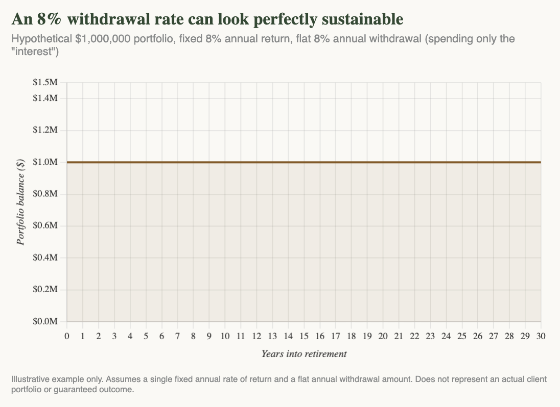
Say a projection assumes an average annual return of 8 percent. On a straight-line basis, an 8 percent withdrawal rate might appear entirely sustainable: the math shows the portfolio holding steady, with you spending only the interest. That looks sound on paper. It is also dangerous in practice, because an average return is not the return you actually experience in any given year. Markets might return 26 percent one year and lose 10 percent the next, and still average out to 8 percent over time. A withdrawal rate that looks fine against the average can erode a portfolio that has to weather a real down year, particularly if that down year happens early. A straight-line projection cannot show you that, because it only ever shows you the average.
A historical backtest takes a different approach. It runs your plan against every real historical period on record, whether that starts in 1966 or 2000 or 2008, and shows how the plan would have performed in each case. This is a meaningful improvement, because it captures real sequences of good years and bad years rather than a smoothed average. Its limitation is that history is a fixed and finite sample. It cannot show you a scenario worse than what has already happened, and it can't be said with certainty that the range of future outcomes will resemble the range of the past.
A Monte Carlo simulation provides a clearer sense of the potential paths forward. Rather than a single scenario, it runs your plan through hundreds or thousands of simulated market scenarios, using assumed returns and a standard deviation for the portfolio, where each instance is built from a randomized sequence of returns drawn from a defined range of statistical outcomes. The result is not one projection, but a wide range of possible dollar outcomes: some paths perform well, some poorly, most land somewhere in between. The probability of success you typically see reported is simply the share of those simulated paths in which the money lasted as long as it needed to.
That number is useful, but it is also fairly abstract on its own. A 90 percent probability of success does not mean the plan will work 90 percent of the time in some literal sense, and it does not mean the remaining 10 percent represents a single, uniform kind of failure. It means that under the assumptions built into the model, 90 percent of the simulated dollar outcomes met the stated goal, while the rest fell short by varying amounts and at varying points along the way. Two plans can both show a 90 percent probability of success and still carry very different real-world risk, depending on how wide the range of outcomes is and how severe the shortfalls look in the paths that miss.
Going back to the 8 percent return and withdrawal example from earlier: while the average scenario would remain the same, the projected range of outcomes in a Monte Carlo simulation would likely reveal a probability of success low enough to raise real concern, depending on the other assumptions built into the plan.
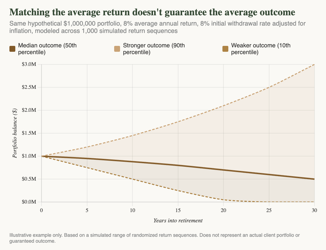
Beyond this, the resulting number does not tell a person what to do, whether it's high or low. It's difficult to say what the real-world difference is between a plan showing a 78 percent probability of success and one showing 83 percent. These numbers are abstract, and they do not inform which account to draw from first, how to respond if portfolio performance falls short, or what to adjust if spending needs change. It is a diagnostic, not a plan. Treating it as something more sets people up with improper expectations of the future, and potentially exposes them to poor strategic decisions. For instance, the range reflected in a Monte Carlo simulation shows scenarios with significantly higher and lower portfolio ending amounts than the median outcome, neither of which is usually the preferred outcome. A plan is how you proceed based on this information and adapt to changing circumstances.
What a Real Plan Actually Looks Like
If the model is a diagnostic rather than a decision, then the plan itself has to be something more than the output of a single simulation. A real plan treats the model as one input among several, informing the strategy rather than standing in for it.
In practice, that starts with how withdrawals are structured. A fixed withdrawal approach, a common example being the 4 percent rule, sets a withdrawal amount in the first year of retirement and simply adjusts it for inflation every year after, regardless of how the portfolio performs. It's simple, but it is also rigid. It cannot respond if markets perform poorly early on, and it leaves no mechanism for spending more if the portfolio is comfortably ahead of plan.
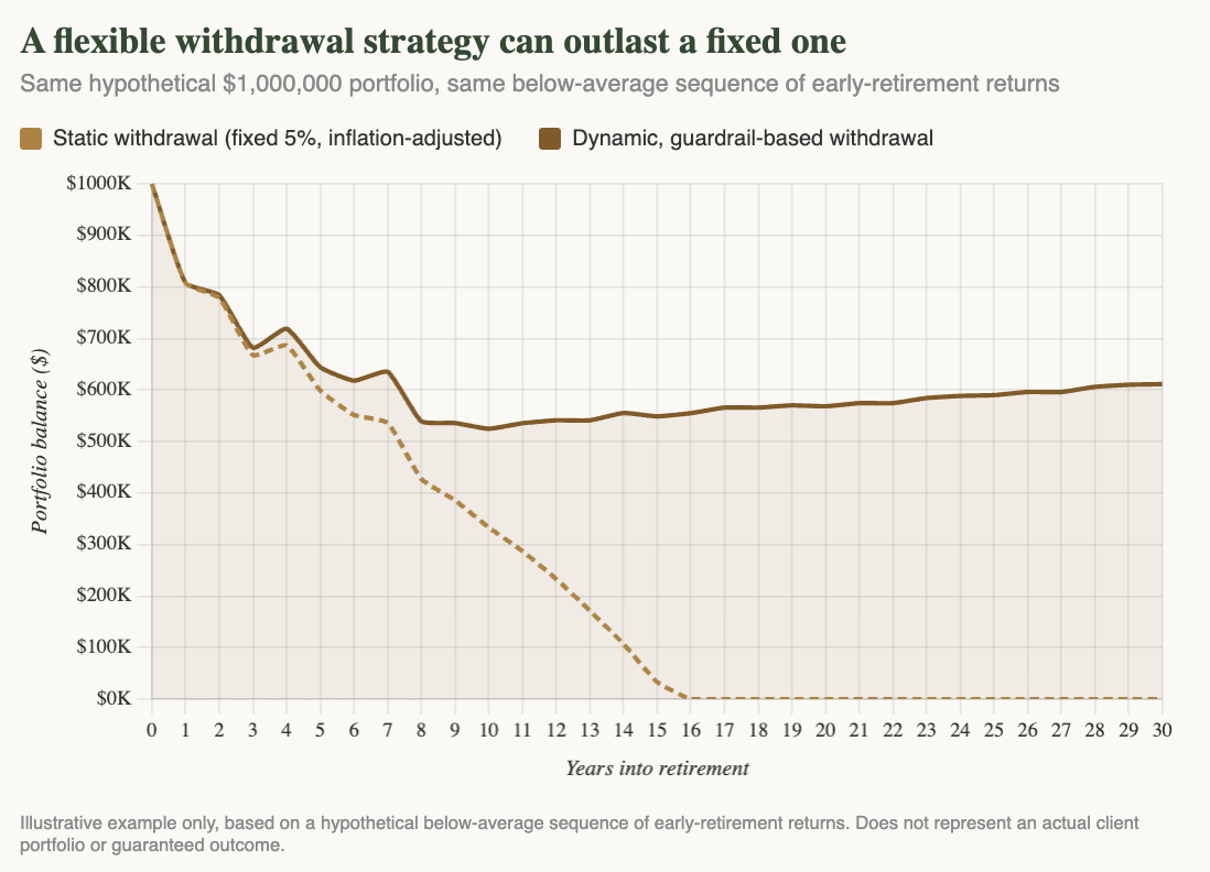
A dynamic withdrawal strategy, guardrail-based for example, is built to respond instead. The approach sets upper and lower thresholds around the withdrawal rate. If the portfolio grows enough that the withdrawal rate drifts meaningfully below its starting point, spending can increase. If a downturn pushes the withdrawal rate meaningfully above its starting point, spending is trimmed for a period, easing pressure on the portfolio during the years it can least afford to be drawn down further. The rules remove some of the guesswork, and some of the emotion, from decisions that are otherwise easy to get wrong in the moment.Flexibility has to extend beyond the withdrawal mechanics themselves. A plan built around a specific set of assumptions at age 60 is not the same plan that should still be in place at 70, particularly once actual market returns, inflation, and spending diverge from what was originally projected, which they inevitably will to some degree. A health event, a change in family circumstances, an earlier or later retirement date than originally intended: each of these is a reason to revisit the plan, not evidence that the original plan failed. The plan that holds up over decades is the one built to be revisited, not the one that got the first draft exactly right.
Why the Assumptions Matter
Whatever form a plan takes, whether a straight-line projection, a historical backtest, or a full Monte Carlo simulation, it is only as sound as the assumptions built into it. A well-constructed model run on unrealistic inputs will still produce a misleading result, and a simpler model built on careful, honest assumptions can be more useful than a sophisticated one that isn't.
The assumptions that matter most are the ones nobody can know in advance: future market returns, future inflation, how long you will actually live, and how spending needs will change over a retirement that could last three decades or longer. There is no way to know these figures with precision today, which means the question is not how to predict them accurately, but how to choose them responsibly.
That argues for a conservative bias. Assuming somewhat lower returns, somewhat higher inflation, and a somewhat longer time horizon than a best-case scenario would suggest builds a margin of safety into the plan from the outset. If reality turns out better than assumed, the plan can be revisited and spending or gifting adjusted upward, a comfortable position to be in. If reality turns out worse than an aggressive set of assumptions projected, the correction required is often a painful one, arriving later in life when there is less time and fewer options to absorb it.
Assumptions are also where stress testing does its work. A plan is not just run once under a base case and left alone. It is tested against a range of specific, adverse conditions: a market downturn in the first several years of retirement, a stretch of inflation well above the assumed rate, an earlier retirement date than intended, or a longer lifespan than the base case assumes. Each of these tests answers a specific question: under what conditions does this plan hold up, and under what conditions does it not.
The Cost of Getting It Wrong
The consequences of skipping this step, or of building a plan on assumptions that were too optimistic to begin with, show up in two different directions, and both carry real costs.
The more familiar risk is running short. A plan built on overly optimistic assumptions, or one that was never stress tested against a genuinely difficult sequence of returns, can look sound for years before the underlying fragility becomes apparent. By the time it does, the corrective options are often limited: reduce spending meaningfully, return to work, or accept a materially different retirement than the one originally planned for. The earlier this risk goes undetected, the fewer good options remain by the time it surfaces.
The less discussed risk runs the opposite direction. A plan built on assumptions that are too conservative, never revisited for years, can produce the same probability-of-success number while quietly steering you toward underspending relative to what you could actually afford. Years of unnecessary austerity, delayed gifting to children or causes that matter to you, experiences postponed and never revisited: these costs are significant, and they come at the expense of your ability to reasonably enjoy your wealth and pursue what matters to you. A plan that is never adjusted upward when circumstances allow it is failing you just as surely as one that runs short.
Both outcomes trace back to the same root cause: a plan treated as a one-time, static exercise, rather than something built to be refined over time.
Beyond Spending: The Strategy Layer
Everything discussed so far speaks to spending: how much, how flexibly, and how the probability of success responds to each. But an effective plan does not stop at spending levels. It also has to weigh a second, deeper layer of strategy. Common examples include when to claim Social Security, whether and when to convert retirement assets to Roth accounts, and in what order to draw from different account types over time.
These decisions rarely have a single correct answer, because doing what looks best on one measure can work against another. Roth conversions are a good example. Converting pre-tax assets to Roth early in retirement can reduce future required distributions and lower lifetime taxes, both of which show up as clear positives in a long-term projection. But paying that conversion tax draws down the portfolio balance in the early years of retirement, exactly when the sequence of returns matters most. Someone who converts aggressively in year one or two of retirement, only to face a market downturn shortly after, has less capital left to absorb that downturn than someone who held off. The long-term tax benefit is real. So is the added near-term risk.
The same balancing act shows up in distribution order and Social Security timing. Delaying Social Security generally increases the eventual benefit, but it also means drawing more heavily from the portfolio in the interim years, which changes the plan's exposure to a poor sequence of returns during exactly the period it can least absorb one. There is rarely a single move that improves every dimension of a plan at once. The most tax-efficient choice is not always the most resilient one, and the choice that produces the highest probability of success on paper is not always the one that best fits your actual risk tolerance or need for certainty.
An effective plan weighs these tradeoffs deliberately rather than optimizing for one number in isolation. That means understanding not just what a given strategy does to lifetime taxes or to a probability of success score, but what it does to the plan's vulnerability in the years that matter most, and making an informed, deliberate decision about how much of one to trade for the other.
What an Effective Plan Actually Looks Like
An effective retirement plan does the modeling. It runs the Monte Carlo simulation, considers the historical record, and understands what a straight-line projection can and cannot tell you. It uses assumptions that are honest about what cannot be known in advance, biased conservatively rather than optimistically, and it stress tests the result against the specific conditions, market downturns, inflation spikes, longer lifespans, that would actually put the plan under pressure. It builds in a withdrawal strategy designed to adapt rather than one that holds rigidly to a single number regardless of what markets or circumstances do.
But the models and the strategy are only the raw material. What they get built into is a decision-making framework, applied specifically to your situation, that tells you what path you are on and what to actually do as circumstances unfold. Markets will not move the way any model assumes. Life will not proceed exactly as planned. The value of an effective plan is not that it predicted the future correctly. It is that it already worked through how you would respond to different outcomes, helping you understand the paths forward and stay confident in your decisions.
That is ultimately what the work produces: not just a strategy, but clarity. Someone working from an effective plan understands where they stand today, what would need to happen for that to change, and what the near-term and long-term implications of their decisions actually are. The specific models and strategy underneath the plan matter. But the measure of whether the plan is actually working is whether it gives you a clear path forward, and a clear sense of how to handle it when reality inevitably diverges from the assumptions.
As always, if you feel your plan could benefit from a revisit or second set of eyes, we are more than happy to discuss how you can take the right steps forward.
Disclosures
This article is provided by McAdam LLC ("McAdam" or the "Firm") for informational purposes only. Investing involves the risk of loss, and investors should be prepared to bear potential losses. Past performance is not indicative of future results and may have been impacted by events and economic conditions that will not prevail in the future. No portion of this article is to be construed as a solicitation to buy or sell any security or the provision of personalized investment, tax, or legal advice. Certain information contained herein is derived from sources believed to be reliable; however, McAdam does not guarantee the accuracy or completeness of such information and assumes no liability for any resulting damages.
Donohue Wealth Management is a DBA of McAdam LLC, an SEC-registered investment adviser. Registration does not imply a certain level of skill or training. Advisory services are offered through McAdam LLC.
Graph 1 (Straight-Line Projection): Illustrative example only. Assumes a single fixed annual rate of return. Does not represent an actual client portfolio or guaranteed outcome.
Graph 2 (Monte Carlo Simulation): Illustrative example only. Based on a simulated range of randomized return sequences. Does not represent an actual client portfolio or guaranteed outcome. Past performance may not be indicative of future results.
Graph 3 (Static vs. Dynamic Withdrawal Strategy): Illustrative example only, based on a hypothetical below-average sequence of early-retirement returns. Does not represent an actual client portfolio or guaranteed outcome.
Sources
Bengen, William P. "Determining Withdrawal Rates Using Historical Data." Journal of Financial Planning, October 1994.
Guyton, Jonathan T., and William J. Klinger. "Decision Rules and Maximum Initial Withdrawal Rates." Journal of Financial Planning, Vol. 19, No. 3, 2006.
Methodology and Assumptions
Graph 1 and Graph 2 use a hypothetical $1,000,000 starting portfolio over a 30-year retirement horizon for illustrative comparison purposes only. Graph 1 assumes a fixed 8% annual return with a flat 8% annual withdrawal, held constant rather than inflation-adjusted, to illustrate a simple "spend only the interest" scenario. Graph 2 illustrates a simulated distribution of outcomes under the same 8% average annual return and 8% initial withdrawal rate, this time inflation-adjusted, rather than actual modeled data; the 50th percentile path falls below the flat outcome shown in Graph 1 due to volatility drag, the compounding effect by which a fluctuating sequence of returns with a given arithmetic average produces a lower typical outcome than a constant return of that same average. Graph 3 illustrates a hypothetical $1,000,000 portfolio subject to a below-average sequence of returns in the first years of retirement, comparing a fixed 5% inflation-adjusted withdrawal against a guardrail-based approach with 10% spending adjustments triggered at 20% deviation from the initial withdrawal rate, consistent with the general structure of the Guyton-Klinger framework. These figures are illustrative only and are not projections or guarantees of any actual portfolio's performance.