
When is the Right Time to Invest?
Executive Summary
There is always a reason to wait. Markets feel too high, or too uncertain, or too fragile. A headline warns of recession; an election looms; a war flares. The instinct to hold off until things settle down is understandable. It is also, by the historical record, expensive.
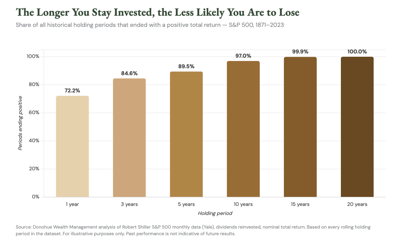
The single most reliable finding in more than 150 years of S&P 500 data is that the probability of earning a positive return rises the longer you stay invested. Over any one-year window since 1871, the market finished higher 72% of the time. Stretch the holding period to ten years and that figure climbs to 97%. At fifteen years it reaches 99.9%, and at twenty years and beyond, every single period in the dataset ended positive. Patience does not guarantee a return in any given year, but over a reasonable horizon it has historically removed the question of whether you would have one at all.
The lesson is not that markets never fall. They fall often and sometimes severely. The lesson is that the cost of trying to avoid those falls, by sitting out and waiting for a better entry point, has been far greater than the cost of simply staying invested and continuing to contribute. This paper looks at three of the worst stretches in market history and shows that an investor who kept buying through them came out ahead, even when the market itself went nowhere.
The Timing Trap
Timing the market means trying to buy before it rises and sell before it falls. It is an appealing idea because it sounds like prudence. In practice it requires being right twice: once on the way out and once on the way back in. Miss either call and the strategy fails.
The deeper problem is that the market's best days tend to cluster near its worst ones, often within the same few weeks. An investor who steps aside during a downturn to “wait for clarity” frequently misses the sharp recovery that follows, because clarity arrives only after the rebound is well underway. The math is unforgiving: a portfolio that misses even a handful of the strongest days over a long period gives back a large share of its total return.
This is why we focus our clients on time in the market rather than timing the market. The first is something you control. The second is something almost no one does well, consistently, over decades.
The Probability of Patience
Consider the holding-period data more closely. Over a single year, the S&P 500 has been a coin flip with a favorable bias: positive about 72% of the time, but with outcomes ranging from a 62% loss to a 140% gain. That is a wide and frightening spread, and it is exactly the volatility that frightens investors out of the market at the wrong moment.
Now extend the horizon. At five years, the share of positive periods rises to 90% and the worst annualized outcome narrows considerably. At ten years, 97% of periods were positive and the worst result was a decline of only about 4% per year. By fifteen years, essentially every period was positive. By twenty, all of them were, with the weakest twenty-year stretch in history still delivering a positive annualized return.
Time does two things at once. It raises the odds of a positive outcome, and it compresses the range of outcomes toward the long-run average. Volatility that is overwhelming over a year becomes manageable over a decade and nearly irrelevant over two. For a pre-retiree with a multi-decade horizon that does not end at the retirement date, this is the central insight: the market's short-term unpredictability is real, but it is also the price of admission for a long-term result that history has rewarded with remarkable consistency.
Crisis Case Study: The Lost Decade
The decade from March 2000 through March 2010 is a great example of when markets can take a while to turn positive. An investor who put $10,000 into the S&P 500 in March 2000, at the very peak of the dot-com boom, and simply held it for ten years would have ended with about $9,575. After a full decade, including reinvested dividends, the money had shrunk. The period earned the nickname “the lost decade” honestly: a buy-and-hold investor lost roughly 4% in total, an annualized return of about negative 0.4%.
But almost no one invests a single lump sum and then adds nothing for ten years. Most people invest the way they earn: steadily, a portion of each paycheck, month after month. Consider an investor who instead spread that same $10,000 evenly across the decade, investing about $83 every month from March 2000 through March 2010.
That investor ended the decade with about $11,118. The same market, the same ten years, the same total dollars invested, and the result flipped from a loss to a gain of roughly 11%. The reason is straightforward. By continuing to buy through the two major declines of the decade, the dot-com collapse and the 2008 financial crisis, the monthly investor accumulated shares at progressively lower prices. When the market was cheap, the fixed monthly contribution simply bought more. Those low-priced shares did the heavy lifting once any recovery came.
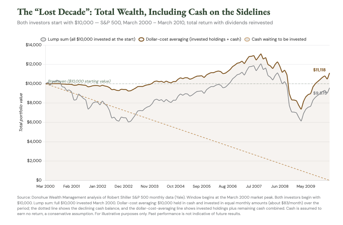
Total portfolio value of $10,000 in the S&P 500 from March 2000 to March 2010, comparing a single lump-sum investment with steady monthly investing. Both investors begin with $10,000; the dollar-cost-averaging total includes cash not yet invested.
The lost decade did not punish investors. It punished investors who stopped. The ones who kept going were rewarded precisely because prices fell.
When History Looked Hopeless
The lost decade is not unique. Two earlier periods looked even more dire in the moment, and both reward the same behavior.
The first is the Great Depression. An investor who bought at the market peak in September 1929 and held for seven years, through the worst economic collapse in modern history, would have seen $10,000 fall to about $7,587, a loss of roughly 24%. Yet an investor who put the same $10,000 in gradually over those seven years, buying steadily as prices cratered to a fraction of their former level, would have ended with about $17,661. The same market that lost a quarter of a lump sum's value turned a stream of monthly investments into a 77% gain, because the buying happened when stocks were at their cheapest in a generation.
The second is the period from 1937 to 1944, which combined a sharp recession in 1937 with the early years of the Second World War. Over those seven years a lump sum invested at the start went essentially nowhere: $10,000 became about $9,873, a total return of negative 1.3%. The market, on a buy-and-hold basis, was flat for seven years. The monthly investor, however, ended with about $13,228, a gain of roughly 32%. This is perhaps the clearest illustration of the principle. The market delivered nothing to someone who bought once and waited, yet delivered a meaningful return to someone who kept investing through a period that went nowhere.
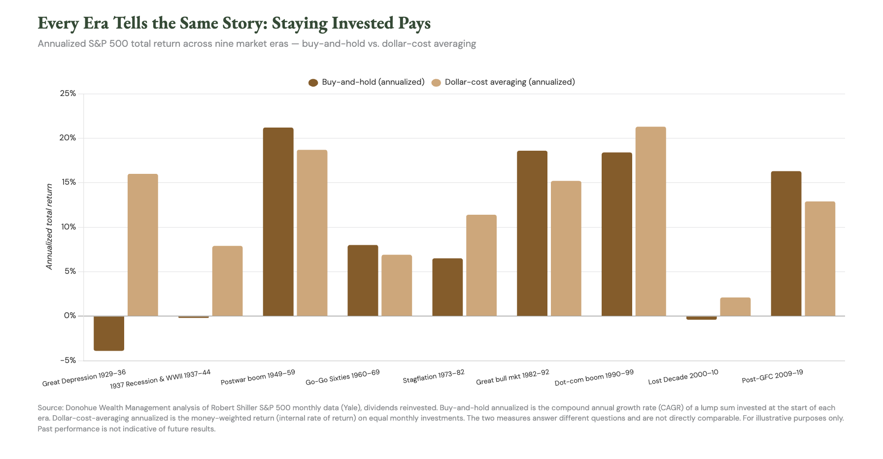
It is worth being precise about why steady investing wins in these particular periods, because the relationship is not universal. Dollar-cost averaging outperforms a lump sum specifically when an investor begins near a market peak and prices then fall or stagnate before recovering. Each of the three crisis eras above fits that description. In strongly rising markets the opposite holds: a lump sum invested early compounds for longer and tends to outperform, which is why eras like the postwar boom, the 1980s and 1990s bull markets, and the post-2009 recovery show higher buy-and-hold figures.
The point is not that one strategy always beats the other. The point is that across nine distinct eras, spanning depression, war, stagflation, and financial crisis, the investor who kept buying ended with a positive result in every single one. Even the worst decades in American financial history were survivable, and frequently profitable, for the investor who simply continued.
What This Means for You
If you are years from retirement, or recently into it with decades of life still ahead, the practical implications are clear.
First, the decision that matters most is not when to invest but whether to keep investing. The historical edge belongs to the participant, not the forecaster.
Second, market declines are not emergencies to be escaped. For anyone still contributing, they are opportunities to accumulate shares at lower prices, exactly the mechanism that rescued returns in every crisis above.
Third, the right time horizon is longer than most people assume. Retirement is not a finish line at which a portfolio is liquidated. A 65-year-old today may need that portfolio to work for another 25 or 30 years, which is precisely the horizon over which the market has never produced a loss.
None of this requires predicting the next recession, the next rate decision, or the next election. It requires the discipline to start, and the patience to stay. Wednesday, or any ordinary day, is the right time to invest, because the value of investing has never come from choosing the perfect moment. It has come from the time that follows.
Let's Talk
If you would like to review how these principles apply to your own portfolio, contribution strategy, and retirement timeline, we would welcome the conversation. Schedule a call with Donohue Wealth Management and we will walk through where you stand and what a disciplined, long-horizon plan looks like for you.
Methodology
Data source. All calculations use the Robert Shiller monthly S&P 500 dataset maintained at Yale University, which provides monthly index levels, dividends, and the Consumer Price Index dating to 1871. This is the standard academic source for long-run U.S. equity analysis. The dataset's dividend and price series run through June 2023; all calculations in this paper fall within that fully sourced window. The index referenced throughout is the S&P 500 (and its historical predecessors as compiled by Shiller).
Total return. Returns are calculated on a total-return basis, meaning dividends are reinvested. We construct a monthly total-return index from the index price level plus the monthly portion of S&P dividends (the trailing annual dividend divided by twelve), compounded month over month. The resulting long-run figures (a nominal annualized total return of about 9.2% and a real, inflation-adjusted return of about 6.9% over the full period) align with established historical estimates, confirming the construction.
Holding-period probability. For each holding period (1, 3, 5, 10, 15, and 20 years) we measure the annualized total return of every possible rolling window in the dataset, then calculate the share that ended positive. For example, the 10-year figure reflects more than 1,700 overlapping 10-year periods.
Buy-and-hold (“lump sum”). A single investment of $10,000 made at the start of the period, held with dividends reinvested to the end. The annualized figure is the compound annual growth rate (CAGR).
Dollar-cost averaging (DCA). Rather than investing the full amount at once, the DCA scenario invests an equal amount every month across the entire period, with dividends reinvested. For a 120-month decade, this means investing $10,000 divided by the number of months, or about $84, at the start of each month. This mirrors how most investors actually contribute: steadily, from ongoing income, rather than in a single lump sum. In the lost-decade illustration, where total portfolio value is shown, the DCA investor is assumed to begin with the full $10,000 in cash and draw it down over the period; cash awaiting investment is assumed to earn no return, a deliberately conservative assumption that understates the DCA result.
DCA annualized return. Because contributions are made gradually, a simple start-to-end growth rate would overstate performance, since most dollars are invested for less than the full period. We instead use the money-weighted return, also known as the internal rate of return (IRR). This is the single annual rate that, applied to each contribution for the actual length of time it was invested, reproduces the ending portfolio value. We solve for the monthly rate at which the present value of all contributions equals the final value, then annualize it. This is the same methodology used in personal rate-of-return reporting. Because buy-and-hold annualized (CAGR) and DCA annualized (IRR) measure different things, one the growth of a single early dollar and the other the average rate earned across a stream of contributions, they are not directly comparable, and the paper does not treat them as such.
Important interpretive note. The DCA results in this paper outperform buy-and-hold because each crisis era studied begins near a market peak, followed by a decline. This is the specific condition under which dollar-cost averaging has an advantage. In steadily rising markets, a lump sum invested earlier generally outperforms, because those dollars compound for longer. The era comparison includes both types of period to present a complete and honest picture.
Sources
Robert J. Shiller. “Online Data: U.S. Stock Markets 1871-Present and CAPE Ratio.” Yale University Department of Economics. Monthly S&P 500 price, dividend, and CPI data. http://www.econ.yale.edu/~shiller/data.htm
Robert J. Shiller. “Irrational Exuberance.” Princeton University Press, 2000; 2nd ed. 2005. (Source of the dataset construction methodology.)
Federal Reserve Bank of St. Louis (FRED). S&P 500 index series (used to confirm recent index levels). https://fred.stlouisfed.org/series/SP500
All return calculations are original analysis by Donohue Wealth Management using the Shiller dataset.
Disclosures
This material is provided for informational and educational purposes only and does not constitute investment, tax, or legal advice. Past performance is not indicative of future results. The information contained herein is believed to be from reliable sources but its accuracy and completeness cannot be guaranteed. All investing involves risk, including the potential loss of principal.
Indexes are unmanaged and cannot be invested in directly. Index returns do not reflect any fees, expenses, or sales charges. The hypothetical examples shown do not represent the performance of any specific investment and do not account for the fees, taxes, or transaction costs that an actual investor would incur, which would reduce returns.
Dollar-cost averaging does not assure a profit and does not protect against loss in declining markets. Because dollar-cost averaging involves continuous investment regardless of price levels, investors should consider their ability to continue making contributions through periods of low price levels.
Historical examples and hypothetical illustrations are provided for educational purposes only and are not intended to predict future market performance or investment outcomes.
Donohue Wealth Management is a DBA of McAdam LLC, an SEC registered investment adviser. Registration does not imply a certain level of skill or training.
Chart data sourced from the Robert Shiller S&P 500 dataset (Yale University) as described in the Methodology section. For illustrative purposes only.